

Recently, the ButterflyMX data team was asked to provide statistics on network bandwidth usage data from our whole fleet of deployed IoT devices. Collecting all of this data and formatting it for convenient access is no easy task — over long periods of time and large volumes of large tables, costs add up.
The original model we used to produce this data had a lot of room for improvement. However, after we poked around and did our research, we found a way to create performance savings that were more than fivefold, from 164 s to 32 s. And as our fleet of devices generates more data, our model will only become more efficient.
So how did we manage that reduction? The answer lies in our embrace of window functions in incremental dbt models. And while you may have heard that these are difficult to implement, you might be able to review how our team implemented them and use them in your own projects.
In this post, we explain what dbt is and what you can use it for. Then, we detail the conditions that made window functions in incremental dbt models the right choice for our data. Finally, we give a dbt incremental model example by walking you through our step-by-step implementation.
This post covers:
- What is dbt?
- Initial conditions: How to make our data usable
- How we dealt with the data
- Our solution: How we used window functions in dbt models
What is dbt?
Before we explain our specific case scenario, let’s go over dbt first and the concepts it relies on.
dbt (data build tool) is an open-source data transformation tool designed to allow any analyst with SQL skills to contribute to data pipelines. It’s used to automate data transformations within a data warehouse and puts in easy-to-reach tools to keep those transformations repeatable and non-destructive. dbt statements are run on schedules and can easily be tested in development environments before being integrated into production workflows.
dbt also simplifies efficiency increases, most importantly by allowing a single model to code for “incremental” and “full-refresh” modes.
Incremental vs. full-refresh
A full refresh will drop the target table and recreate it with newly transformed data based on the entirety of the source table or tables. In contrast, a dbt incremental model will only add to the target table transformed data from the source tables that are new since the last dbt run, incremental or otherwise.
The incremental dbt model is run most of the time and the full-refresh model can correct any blips that do occur on a daily, weekly, or less frequent basis.
Initial conditions: How to make our data usable
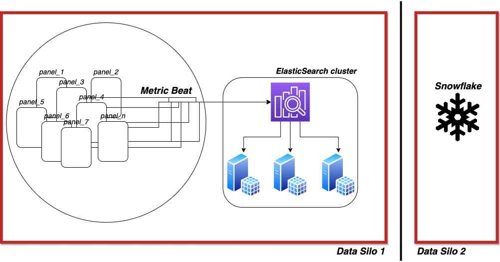
To reiterate, we were tasked with statistics on network bandwidth usage data from our fleet of deployed IoT devices. We collect this data using Metricbeat agents deployed on our IoT devices and send it to our Elasticsearch cluster.
But we wanted to make some changes to the raw data to make it easier to access.
First, our strategy on the data team is to provide “self-service” data access as much as possible to all our internal clients. We want to spend our time building dashboards and portals that free our data so that anyone at the company can find answers to their questions themselves, via tools that match their skillsets, rather than relying on data specialists or even technical people at all.
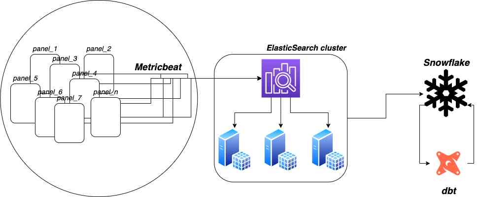
We selected Sigma as a dashboarding tool resting on a Snowflake data warehouse to serve these needs. However, the data in Elasticsearch is stored in JSONs. We need to get the data into Snowflake so that Sigma can interact with it, and so that we can enrich this data with data from other tables. We need relational data.
What other conditions are we setting for our data?
Second, it’s not cost-effective to store raw data indefinitely, especially in a ‘hot’ state in our Elasticsearch cluster. In the case of network bandwidth utilization data, Elasticsearch’s data retention period is insufficient to detect longer-term and cyclical patterns in the data. Longer retention, and therefore aggregation, is necessary to discover patterns and make business decisions. We need summarized data in Snowflake.
Third and finally, and most pertinently to this post’s theme of window functions, the raw bandwidth usage data arrives as cumulative usage since device boot, rather than deltas. We receive updates many times per hour. So, for example, at 10:00 we might have a usage of ‘103,000,000’ b for one device, ‘105,000,000’ at 10:30, and ‘108,000,000’ at 11:00, meaning the total usage for that hour was 5MB. We need transformations on the raw data.
To summarize, we wanted our network usage data to be:
- Relational and easily enriched with data from other tables
- Retained for long periods of time
- Transformed and represented as a change per hour rather than cumulative usage
Watch how ButterflyMX works:
How we dealt with this data
Given the goals that we started out with, we wanted to set up guidelines for ourselves that would allow us to represent the data the way we wanted to.
So, we decided to make this data readable by following these two conditions:
- Using a dbt incremental model and a full-refresh model simultaneously
- Converting the cumulative bandwidth usage data into deltas representing hourly usage
These conditions mean that we want an ELT (extract-load-transform) pipeline to bring the data out of Elasticsearch and into the Snowflake data warehouse. And we want dbt to manage and automate the transformations on it.
Using a dbt incremental model and a full-refresh model simultaneously
We have a large and growing IoT fleet, with many new documents arriving to Elasticsearch every second. The extract and load portions of the ELT pipeline will eliminate some of this volume, and dbt and Snowflake are highly optimized systems. However, costs add up over long periods of time.
So, we settled on an hourly update cadence and an incremental model with the idea that it will:
- Save on direct costs in Snowflake
- Reduce runtime in dbt Cloud
- Reduce latency during work hours
But automation glitches, a fat-finger mistake that’s later corrected, or other bugs could introduce duplicates or otherwise bad data. For this reason, we also chose to implement full data refreshes from the complete raw data source on a weekly cadence.
Convert the cumulative bandwidth usage data into deltas representing hourly usage
Because we wanted to use an incremental model, we wanted to store changes in cumulative bandwidth as deltas representing hourly usage.
See the HOURLY_BYTES_IN column in the table below for an example:
| DEVICE_ID | TIME_BUCKET_KEY | CUMUL_BYTES_IN | HOURLY_BYTES_IN |
|---|---|---|---|
| 1113 | 2022-02-29 01:00:00.000 | 239168200 | NULL |
| 1113 | 2022-02-29 02:00:00.000 | 240713439 | 1545239 |
| 1113 | 2022-02-29 03:00:00.000 | 242319214 | 1605775 |
| 1116 | 2022-02-29 01:00:00.000 | 1429681671 | NULL |
| 1116 | 2022-02-29 02:00:00.000 | 1431478090 | 1796419 |
| 1116 | 2022-02-29 03:00:00.000 | 1433333243 | 1855153 |
Our solution: How we used window functions in dbt models
Let’s sum up first:
By now, you understand that the data from our devices comes in a cumulative format — but we wanted to represent this data as an hour-by-hour change instead. And we wanted to put this data into tables that are compatible with both incremental and full-refresh methods of adding data.
Here’s how we got there with the help of window functions and dbt.
Follow along with our step-by-step solution:
- Setting up the window functions
- Making our incremental models compatible with window functions
- Using dbt to allow for full refreshes within an incremental model
1. Setting up the window functions
For every row in a table, we:
- Group by each individual device
- Order by the timestamp of the information
- Calculate the data consumed in the past hour by subtracting the previous row’s cumulative usage from the current row’s cumulative usage
We accomplish all this using a window function. Specifically, we use the LAG function:
    SELECT
    bytes_in - LAG(bytes_in, 1, NULL) OVER (PARTITION BY device_id ORDER BY time_bucket_key)
    FROM bandwidth_data
The OVER keyword and the phrase within the parentheses that follow are the core syntax of the window function. We can partition by one or many columns and order by one, none, or many others. In this case, we only need to partition the data by the device_id column and order it only by the timestamp column.
The LAG keyword allows us to manipulate the value of a column from a prior row in conjunction with values from the current row.
The function’s three arguments are:
- Column of interest
- Number of rows to look back (1 to look at the previous row)
- Default value to return if the lag looks for a row that doesn’t exist (i.e., looking for a row before the first row of the table)
2. Making our incremental models compatible with window functions
Hang on, window functions are incompatible with incremental models.
…or are they?
As we attempted to implement our solution, we found using window functions within incremental models to be challenging, and turned to the online community for answers. We discovered that the use of window functions in incremental models is very commonly considered difficult due to the additional context required by the window function, which drives up the complexity of the model.
Incremental models are meant to sift out only the most recent values, and window functions by definition require more context than a single row per key.
However, we can solve this problem by using another window function in a nested subquery to add a rank column. We will partition by the individual devices, order by the timestamp, and then filter out all the rows with a rank greater than two:
    SELECT
    bytes_in - LAG(bytes_in, 1 ,0) OVER (PARTITION BY device_id ORDER BY time_bucket_key)
    FROM (
        SELECT *,
                RANK() OVER (PARTITION BY device_id ORDER BY time_bucket_key DESC) AS rank
              FROM bandwidth_data
              QUALIFY rank < 3 )
Now we have the two most recent rows for each column. We apply our other window function to transform the cumulative column into deltas, and finally use a subsequent CTE (common table expression) to get only the very latest data available and push them into the model table.
    WITH window_table AS (
        SELECT
            bytes_in - LAG(bytes_in, 1 ,0) OVER (PARTITION BY device_id ORDER BY time_bucket_key)
        FROM (
            SELECT *,
                    RANK() OVER (PARTITION BY device_id ORDER BY time_bucket_key DESC) AS rank
            FROM bandwidth_data
            QUALIFY rank < 3 )
    ),

    final AS (
        SELECT
            bytes_in
        FROM window_table
        WHERE rank = 1)

    SELECT * FROM final
We now have a model implementing window functions that adds only one or zero rows of data per device to the table every time it is run. Victory!
3. Using dbt to allow for full refreshes within an incremental model
But wait, won’t this inhibit the use of a full refresh model?
We now have an incremental model that can run every hour and add only the latest data to the final table. But at first glance, using an incremental model and a full refresh model at the same time doesn’t seem possible.
While incremental models typically share a SELECT statement with the full refresh model, containing only a WHERE clause in the incremental wrapper, our model has entire complex SELECT statements in the incremental wrapper and requires totally distinct statements for a full refresh. Does this mean we can’t have a weekly/monthly full refresh of the model?
In short, no. And while dbt is incremental in this case, here’s what we did to allow for full refreshes as well.
In addition to if is_incremental statements, the Jinja framework in dbt also supports if not is_incremental code blocks, which function as expected. Instead of having a small portion of a single SELECT wrapped in an if is_incremental statement, we have two whole SELECTs, one for if is_incremental and one for if not is_incremental:
    WITH window_table AS (
        SELECT


        {% if is_incremental() %}

            bytes_in - LAG(bytes_in, 1 ,0) OVER (PARTITION BY device_id ORDER BY time_bucket_key)
        FROM (
            SELECT *,
                    RANK() OVER (PARTITION BY device_id ORDER BY time_bucket_key DESC) AS rank
            FROM bandwidth_data
            QUALIFY rank < 3 )

        {% endif %}

        {% if not is_incremental() %}

        *
        from bandwidth_data

        {% endif %}
    ),

    final AS (
        SELECT
            bytes_in
        FROM window_table
        WHERE rank = 1)

    SELECT * FROM final
The result is a model that is significantly more complex than the typical incremental dbt model. However, the final file is only about 100 lines of code, nearly all in ANSI SQL, which we feel is an acceptable level of complexity.
Summary
While incremental models implementing window functions will probably be more complex than most of your other dbt models, they’re unlikely to be a barrier to entry for new players on your analytics team.
dbt is a very powerful tool — rather than burdening your project with new limitations, it should be thought of as powerful enough to break down old ones.


Author’s Bio:
Sean Smith is a data engineer at ButterflyMX, breaking down data silos using Python and SQL. He was until recently skeptical about dbt, but is now an evangelist.